Introduction

Source:

Dataset, Drugs Categorization, Effect on Body

Problem:

Based on the effects given to the body, psychotropic substances are, at least, classified into three groups of stimulants, depressants, and hallucinogens. While stimulants affect the body by increasing the alertness and confidence of the consumers, depressants bring a relaxing effect and reduce the concentration of consumers. Alcohol, caffeine, and nicotine are psychotropic substances that are commonly found in societies and are available in beverages and cigarettes. This study aims to segment the consumer based on their demography and personality profile by applying K-Means clustering.

Data Description

The dataset contains 32 columns of data that consists of background, personality, and last intake of 19 drugs from 1885 participants. These 32 columns are id, age, sex, education, country, ethnicity, neuroticism, extraversion, openness, agreeableness, conscientiousness, impulsiveness, sensation seeing, alcohol, amphetamines, amyl nitrite, benzodiazepine, caffeine, cannabis, chocolate, cocaine, crack, ecstasy, heroin, ketamine, legal highs, LSD, methadone, magic mushrooms, nicotine, semeron, volatile substance.

All the values presented in the dataset have been encoded to indicate the classes of each variable so that data encoding is not required. Below is description of drugs intake:

CL0 : Never Used
CL1 : Used over a Decade Ago
CL2 : Used in Last Decade
CL3 : Used in Last Year
CL4 : Used in Last Month
CL5 : Used in Last Week
CL6 : Used in Last Day

Data Preparation

import pandas as pd
df = pd.read_csv('Dataset/drug_consumption.data',header=None)

#check for null value
df.isna().any()
#check for any duplicate
df[df.duplicated()]
#check for data type
df.dtypes

Output finds no null and duplicated values, so the dataset is ready for exploration.

feature = df.iloc[:,:13]
label = df.iloc[:,13:]

Since data type in the label is in an object, so it needs to be encoded into an integer so CL0->0, CL1->1, and so on.

from sklearn.preprocessing import LabelEncoder

laben = LabelEncoder()
for i in range(0,len(label.columns)):
    label.iloc[:,i] = laben.fit_transform(label.iloc[:,i])
label.head()

After assigning features and labels of the data, create a data frame of alcohol, caffeine, and nicotine consumption in variable df_all.

#Set Dataframe
df_all = pd.concat([feature, label.iloc[:,[0,4,16]]], axis=1, join="inner")

Then, the data is filtered for maximum last intake in a week so the value in drugs column is filtered by 5 and 6

df_alc = df_all[(df_all['alcohol'] == 6) | (df_all['alcohol'] == 5)] 
df_caf = df_all[(df_all['caffeine'] == 6) | (df_all['caffeine'] == 5)]
df_nic = df_all[(df_all['nicotine'] == 6) | (df_all['nicotine'] == 5)]

Of the 13 features available in the dataset, the features utilized for clustering in this project are age, education, extraversion, and openness.

feat_alc = df_alc.iloc[:,[1,3,7,8]]     #Select age, education, extraversion, openness
label_alc = df_alc['alcohol']

feat_caf = df_caf.iloc[:,[1,3,7,8]]     #Select age, education, extraversion, openness
label_caf = df_caf['caffeine']

feat_nic = df_nic.iloc[:,[1,3,7,8]]      #Select age, education, extraversion, openness
label_nic = df_nic['nicotine']

K-Means Clustering

import matplotlib.pyplot as plt
from kneed import KneeLocator
from sklearn.datasets import make_blobs
from sklearn.cluster import KMeans
from sklearn.metrics import silhouette_score
from sklearn.preprocessing import MinMaxScaler

Call the feature and label that will be modeled

drug = 'Alcohol'       #Change it to Caffeine or Nicotine
feature = feat_alc     #Change it to feat_caf or feat_nic
label = label_alc      #Change it to feat_caf or feat_nic

c_feat = feature.nunique()
x_label_demo = feature.columns[0]
y_label_demo = feature.columns[1]
x_label_pers = feature.columns[2]
y_label_pers = feature.columns[3]

Before modeling, features still need to be scaled for clustering

scaler = MinMaxScaler()
scaled_features = scaler.fit_transform(feature)

If the number of clusters is unknown, then the optimum k-value can be determined through the elbow method

#Find Optimum Cluster
plt.figure()

kmeans_kwargs = {"init": "random", "n_init": 11, "max_iter": 300, "random_state": 42}

k = range(1, 11)
sse = []

for i in k:
    kmeans = KMeans(n_clusters=i, **kmeans_kwargs)
    kmeans.fit(scaled_features)
    sse.append(kmeans.inertia_)
    
kl = KneeLocator(k, sse, curve="convex", direction="decreasing")
n_clust = kl.elbow
n_clust


plt.plot(k, sse, color='darkgreen')

plt.plot(k[n_clust-1], sse[n_clust-1], 'ro', color='greenyellow', markersize=15)
plt.annotate('Best k value',
             xy=(k[n_clust-1], sse[n_clust-1]),
             xytext = (5, 2000),
             arrowprops = dict(facecolor = 'black', shrink=0.1)
            )
plt.xticks(k)
plt.title(f'{drug} Elbow Method')
plt.xlabel("Number of Clusters")
plt.ylabel("SSE")
plt.show()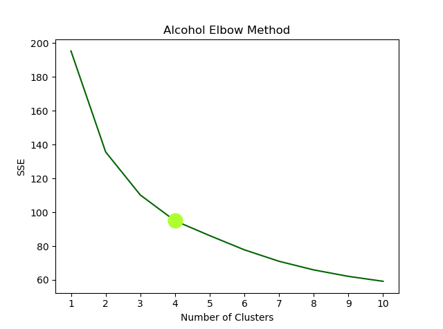

Train the model

scaled_features, label = make_blobs(n_samples=len(scaled_features), centers = n_clust, n_features = 4, random_state=42) #Number of data groups in first feature

kmeans = KMeans(init="random", n_clusters=n_clust, n_init=10, max_iter=300, random_state=42)
kmeans.fit(scaled_features)
drug_clust= kmeans.predict(scaled_features)
inertia = kmeans.inertia_
centers = kmeans.cluster_centers_
iter_ = kmeans.n_iter_

Plot the cluster result. Here the features are divided into two categories, demography and personality.

fig = plt.figure(figsize=(12,6))

plt.subplot(1,2,1) #Demography Features
sct1 = plt.scatter(scaled_features[:,0], scaled_features[:,1], c=drug_clust, s=20, cmap='summer')
plt.scatter(centers[:,0], centers[:,1], color='greenyellow', s=500, alpha=0.5)
plt.title(f'Clustering {drug} Demography')
plt.xlabel(x_label_demo)
plt.ylabel(y_label_demo)
plt.legend(*sct1.legend_elements(), title='clusters',loc='best')

plt.subplot(1,2,2) #Personality Features
sct2 = plt.scatter(scaled_features[:,2], scaled_features[:,3], c=drug_clust, s=20, cmap='summer')
plt.scatter(centers[:,2], centers[:,3], color='greenyellow', s=500, alpha=0.5)
plt.title(f'Clustering {drug} Personality')
plt.xlabel(x_label_pers)
plt.ylabel(y_label_pers)
plt.legend(*sct2.legend_elements(), title='clusters',loc='best')

plt.show()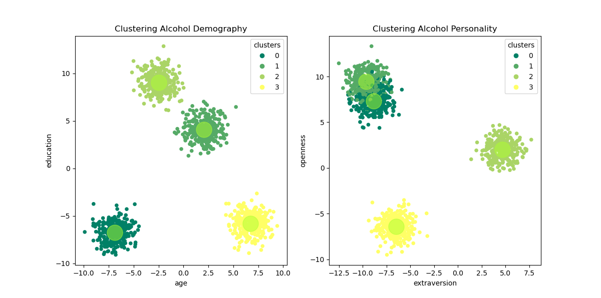

fig = plt.figure()

silhouette_coefficients = []

for k in range(2, 11):
    kmeans = KMeans(n_clusters=k, **kmeans_kwargs)
    kmeans.fit(scaled_features)
    score = silhouette_score(scaled_features, kmeans.labels_)
    silhouette_coefficients.append(score)

plt.plot(range(2, 11), silhouette_coefficients,  color='darkgreen')
plt.xticks(range(2, 11))
plt.xlabel("Number of Clusters")
plt.ylabel("Silhouette Coefficient")
plt.title(f'Silhouette {drug} Clustering ')
plt.show()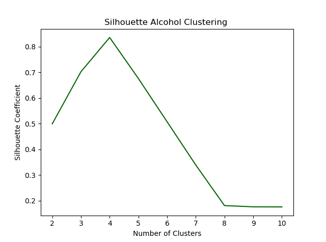

Since the k-value applied is based on the results of the elbow method, the evaluation of the silhouette coefficient shows the maximum score of the related k-value

Discussion and Conclusion

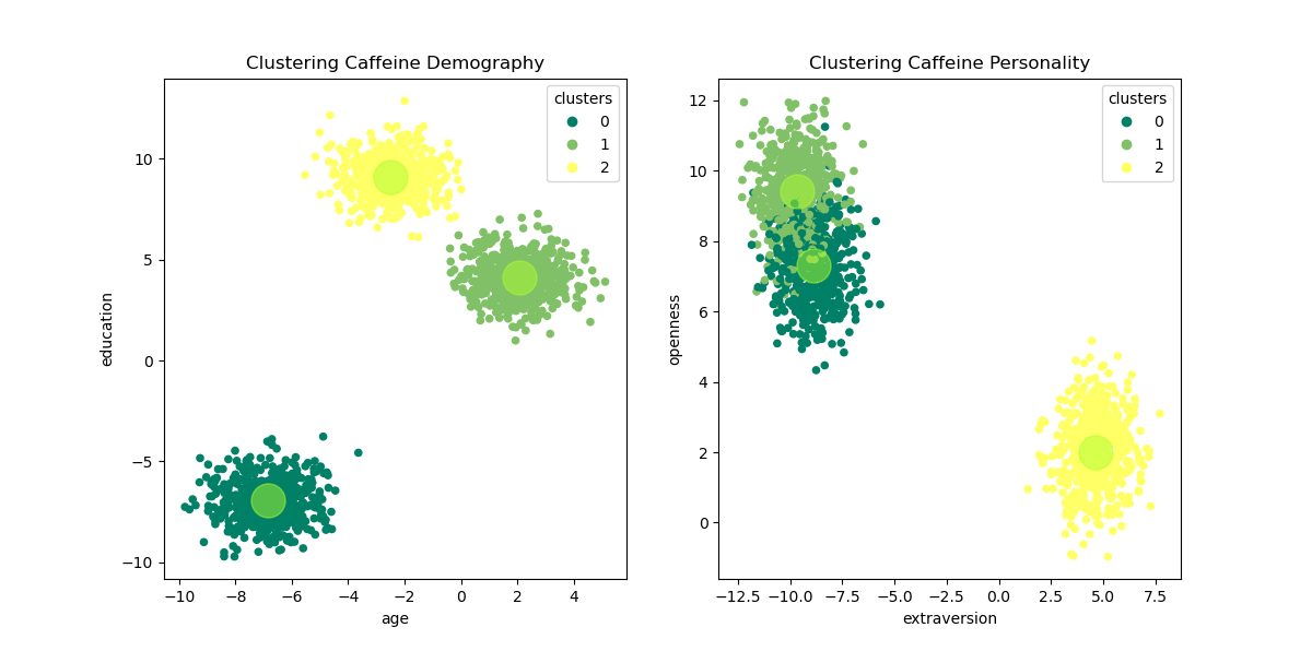
All the K-Means Clustering steps are repeated for caffeine and nicotine. Hence, there will be 3 figures of consumers profile clustering to be compared, as follow:

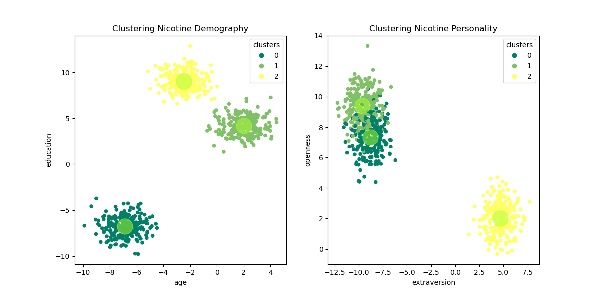
The table below is describe the consumer’s profile for each cluster of each substance

Substances	Profile	Cluster 0	Cluster 1	Cluster 2	Cluster 3
Alcohol	Demography	Low education, Low age group	High education, Middle age group	High education, Middle age group	Low education, High age group
Caffeine	Demography	Low education, Low age group	High education, Middle age group	High education, Middle age group	x
Nicotine	Demography	Low education, Low age group	High education, Middle age group	High education, Middle age group	x
Alcohol	Personality	High openness, Low extraversion	High openness, Low extraversion	Middle openness, High extraversion	Low openness, Middle extraversion
Caffeine	Personality	High openness, Low extraversion	High openness, Low extraversion	Middle openness, High extraversion	x
Nicotine	Personality	High openness, Low extraversion	High openness, Low extraversion	Middle openness, High extraversion	x

From the pictures above, it can be inferred that:

1. The clustering of alcohol consumers has divided the consumer into 4 groups of profiles while the consumer profiles of caffeine and nicotine are divided into 3 groups

2. Profiling of alcohol consumers shows that consumers with low levels of education tend to have personalities with lower extraversion, while consumers with higher education levels have higher levels of openness.

3. As stimulant substances, the clustering of caffeine and nicotine consumers’ profiles shared the same pattern, where demographically the consumers come from young and middle age groups with diverse educational backgrounds. While in personality, the consumers either have a high level of openness or a high level of extraversion.

To conclude, clustering of backgrounds and personalities of alcohol, caffeine, and nicotine consumers has supported for profiling of these psychotropic substances consumers.